Examining the Louvre

“The unexamined life is not worth living” - Plato
Part 1 of ‘Graphing the Louvre’ was all about modeling the “Louvre Online Collection Database” as a Graph, using Neo4j. Part 2 was all about profiling the Graph for some quick Facts & Figures. Here in Part 3, we’re taking it one level higher by employing Graph Data Science algorithms to support our drawn inferences.
While we’re still at analyzing the ‘Painting’ Collection at the Louvre, (read: because I clearly haven’t tagged the ‘Exhibit’ Nodes with the really large ‘Objects’ and ‘Drawings & Prints’ Collections from the Louvre Collections site yet), let’s examine similar Artists. I found this interesting visual that explains how one could study the work of varied Artists and draw inspiration from, in their own art-projects.

Now of the many characteristics outlined here, we’ve got data on the Artist Origin & Occupation, Genre & Movement (Social / Cultural Influences), Materials & Techniques, along with Features that could possibly represent Composition / Mood / Atmosphere / Visual Key Elements.
We’re going to start with a simple Native projection of our scoped data in memory, followed by application of the classic Node Similarity algorithm on the projected in-memory graph.
CALL gds.graph.create(
    'artists&Paintings',
    ['Artist', 'Painting', 'Country', 'Occupation', 'Genre', 'Movement', 'Period', 'Place', 'Feature', 'Material', 'Technique'],
    ['CREATOR', 'COUNTRY', 'OCCUPATION', 'GENRE', 'MOVEMENT', 'PERIOD', 'PLACE', 'FEATURE', 'MATERIAL', 'TECHNIQUE']
);
We’re going to stream the results of Node Similarity for one Artist, say ‘Leonardo da Vinci’, to see what it looks like.
CALL gds.nodeSimilarity.stream('artists&Paintings',
{degreeCutoff: 5,
similarityCutoff: 0.1,
topK:25})
YIELD node1, node2, similarity
WHERE node1 <> node2 AND gds.util.asNode(node1).wikiID = 'Q762'
WITH gds.util.asNode(node1).name AS artist1Name,
gds.util.asNode(node1).wikiID as artist1WikiID,
gds.util.asNode(node1).dateOfBirth AS artist1DOB,
gds.util.asNode(node2).name AS artist2Name,
gds.util.asNode(node2).wikiID AS artist2WikiID,
gds.util.asNode(node2).dateOfBirth AS artist2DOB,
similarity,
[(a:Artist)-[:MOVEMENT]->(m:Movement) WHERE ID(a)=node2|m.movement] AS movement,
[(a:Artist)-[:COUNTRY]->(c:Country) WHERE ID(a)=node2|c.countryEN] AS country
ORDER BY similarity DESC
RETURN artist1Name AS artistName, artist1WikiID AS artistWikiID, artist1DOB AS artistDOB, COLLECT(artist2Name) AS similarArtists,  apoc.coll.toSet(apoc.coll.flatten(COLLECT(movement))) AS movement, apoc.coll.toSet(apoc.coll.flatten(COLLECT(country))) AS country,
apoc.coll.toSet(apoc.coll.flatten(COLLECT(artist2DOB))) AS DOB
I must say I am pretty amazed to see what it shows, ‘Michelangelo’ and ‘Raphael’ both figuring in there among what are the early and high Renaissance period Artists of the time. If we could get to cleansing the data around Artist dates’ of birth from the many formats the Louvre has documented them to be (plain dates, years, month/year, approximate year range, text etc.), it would allow us to filter on them using Cypher projection if we were only interested in say, analyzing Artists belonging to certain period(s). I’d like to see how this compares with another algorithm from the set, (and the original plan was to use Cosine Similarity with embeddings computed using either FastRP/Node2Vec/GraphSAGE but that didn’t work as planned from my Node properties all being ‘String’ data type). So, what we’re then left to do is to compute custom embeddings from the underlying Graph structure and persist them as Node properties that we could then feed to the Cosine Similarity algo.
CALL apoc.periodic.iterate(
"MATCH (a:Artist)
RETURN a,
[(a)-[:COUNTRY]->(ac:Country)|ID(ac)]+[(a)-[:OCCUPATION]->(ao:Occupation)|ID(ao)]+
[(a)-[:GENRE]->(ag:Genre)|ID(ag)]+[(a)-[:MOVEMENT]->(am:Movement)|ID(am)]+
apoc.coll.toSet([(a)<-[:CREATOR]-(p:Painting)-[:PERIOD]->(pp:Period)|ID(pp)])+
apoc.coll.toSet([(a)<-[:CREATOR]-(p:Painting)-[:PLACE]->(pl:Place)|ID(pl)])+
apoc.coll.toSet([(a)<-[:CREATOR]-(p:Painting)-[:FEATURE]->(pf:Feature)|ID(pf)])+
apoc.coll.toSet([(a)<-[:CREATOR]-(p:Painting)-[:MATERIAL]->(pm:Material)|ID(pm)])+
apoc.coll.toSet([(a)<-[:CREATOR]-(p:Painting)-[:TECHNIQUE]->(pt:Technique)|ID(pt)])+
apoc.coll.toSet([(a)<-[:CREATOR]-(p:Painting)-[:GENRE]->(pg:Genre)|ID(pg)])+
apoc.coll.toSet([(a)<-[:CREATOR]-(p:Painting)-[:MOVEMENT]->(po:Movement)|ID(po)]) AS list",
"SET a.embedding = list",
{batchSize:1000, parallel:true})
Now, we could well have fed these embeddings directly in the procedure call to Cosine Similarity itself (instead of having had to persist them on the ‘Artist’ Nodes), however, Cosine Similarity is only calculated over non-NULL dimensions and the algo procedure expects same-length lists for all items as input, failing which, it would trim the longer lists to the length of the shortest list in the data set, resulting in loss of data. Now since not all ‘Artist’ or ‘Painting’ Nodes would have a relationship to each of the scoped characteristic Nodes, we’ll need to pad individual item lists with ‘NaN’ to denote missing values, such that all item lists are of uniform length. We then run Cosine Similarity over previously computed ‘Artist’ Node embeddings, for the same Artist in question, making for a comparison of results.
MATCH (n:Artist)
WHERE NOT n.name = 'ANONYME'
WITH max(size(n.embedding)) AS maxEmbedding
MATCH (a:Artist)
WHERE NOT a.name = 'ANONYME'
WITH a, a.embedding + [x IN range(0, (maxEmbedding-size(a.embedding))-1)|gds.util.NaN()] AS list
WITH {item:ID(a), wikiID:a.wikiID, weights:list} AS artistData
WITH collect(artistData) AS artists
WITH artists,
     [value IN artists WHERE value.wikiID IN ["Q762"] | value.item ] AS sourceIds
CALL gds.alpha.similarity.cosine.stream({
 data: artists,
 sourceIds: sourceIds,
 similarityCutoff: 0.75,
 degreeCutoff: 75,
 topK: 50
})
YIELD item1, item2, similarity
WITH gds.util.asNode(item1).name AS artist1Name,
gds.util.asNode(item1).wikiID as artist1WikiID,
gds.util.asNode(item1).dateOfBirth AS artist1DOB,
gds.util.asNode(item2).name AS artist2Name,
gds.util.asNode(item2).wikiID AS artist2WikiID,
gds.util.asNode(item2).dateOfBirth AS artist2DOB,
similarity,
[(a:Artist)-[:MOVEMENT]->(m:Movement) WHERE ID(a)=item2|m.movement] AS movement,
[(a:Artist)-[:COUNTRY]->(c:Country) WHERE ID(a)=item2|c.countryEN] AS country
ORDER BY similarity DESC
RETURN artist1Name AS artistName, artist1WikiID AS artistWikiID, artist1DOB AS artistDOB, COLLECT(artist2Name) AS similarArtists,  apoc.coll.toSet(apoc.coll.flatten(COLLECT(movement))) AS movement, apoc.coll.toSet(apoc.coll.flatten(COLLECT(country))) AS country,
apoc.coll.toSet(apoc.coll.flatten(COLLECT(artist2DOB))) AS DOB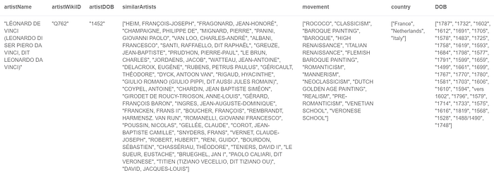
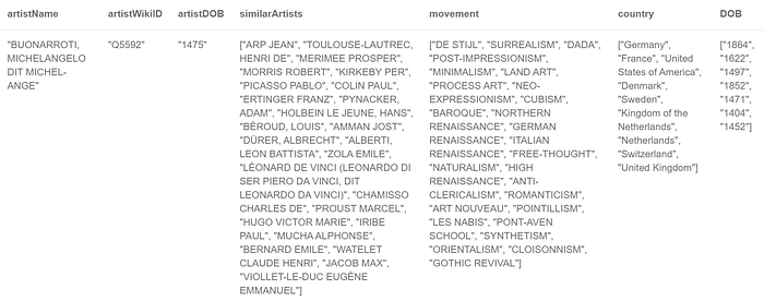
What an interesting ensemble in there! No ‘Michelangelo’, but there’s ‘Raphael’ (1483). ‘Nicolas Poussin’ (1594) shows, and from what’s documented, he studied the works of Renaissance and Baroque painters, especially ‘Raphael’, who had a powerful influence, on his style. ‘Jean-Baptiste-Camille Corot’ (1796) shows, who was exposed to the principles of the French Neoclassic tradition, as exemplified in the works of French Neoclassicist ‘Nicolas Poussin’. Rembrandt (1606) (!) figures too, who was considerably influenced by the work of Italian masters and Netherlandish artists, who studied in Italy, like ‘Peter Paul Rubens’, who also figures alongside! And while we’re at it, Rembrandt’s Night Watch was in the news recently for those of you interested. ‘Théodore Géricault’ (1791) choose to study at the Louvre, where from 1810 to 1815 he copied paintings by ‘Rubens’, ‘Titian’, and ‘Rembrandt’, all of whom figure alongside! … and last but not the least, ‘Eugene Delacroix’, whom I talked of in Part 2. Would we need more a validation of our results? I reckon not.
Let’s look at what ‘Michelangelo’ brings up.
Well, it does show ‘Leonardo da Vinci’, which is surefire validation but Pablo Picasso? erm… also among a whole others I don’t quite recognize. I was reading about the Sistine Chapel, among Michelangelo’s most renowned works of art, and thought maybe it’d be good to see whether there were affinity between the Artists who painted the Sistine Chapel alongside him.

MATCH (n:Artist)
WHERE n.wikiID IN ['Q5592','Q5827','Q5669','Q2311437','Q29447','Q7031','Q191423']
WITH max(size(n.embedding)) AS maxEmbedding
MATCH (a:Artist)
WHERE a.wikiID IN ['Q5592','Q5827','Q5669','Q2311437','Q29447','Q7031','Q191423']
WITH a, a.embedding + [x IN range(0, (maxEmbedding-size(a.embedding))-1)|gds.util.NaN()] AS list
WITH {item:ID(a), weights:list} AS artistData
WITH collect(artistData) AS artists
CALL gds.alpha.similarity.cosine.stream({
 data: artists,
 similarityCutoff: 0.75,
 degreeCutoff: 10
})
YIELD item1, item2, similarity
WITH gds.util.asNode(item1).name AS artist1Name,
gds.util.asNode(item1).wikiID as artist1WikiID,
gds.util.asNode(item1).dateOfBirth AS artist1DOB,
gds.util.asNode(item2).name AS artist2Name,
gds.util.asNode(item2).wikiID AS artist2WikiID,
gds.util.asNode(item2).dateOfBirth AS artist2DOB,
similarity,
[(a:Artist)-[:MOVEMENT]->(m:Movement) WHERE ID(a)=item2|m.movement] AS movement,
gds.util.asNode(item2).placeOfBirth AS placeOfBirth
ORDER BY similarity DESC
RETURN artist1Name AS artistName, artist1WikiID AS artistWikiID, artist1DOB AS artistDOB, COLLECT(artist2Name) AS similarArtists,  apoc.coll.toSet(apoc.coll.flatten(COLLECT(movement))) AS movement, COLLECT(placeOfBirth) AS placeOfBirth,
apoc.coll.toSet(apoc.coll.flatten(COLLECT(artist2DOB))) AS DOB
I think it’s simply amazing that all of the involved Artists (that we chose to examine) depict strong affiliation to ‘Michelangelo’.

We have enough reason to run Node Similarity and mutate our in-memory graph with a SIMILARITY relationship and associated score, that we could then employ to detect communities of like-minded Artists. Note: Cosine Similarity does not have a mutate function being in the alpha tier at this time of writing.
CALL gds.nodeSimilarity.mutate('artists&Paintings',
{degreeCutoff: 5,
similarityCutoff: 0.1,
topK:25,
mutateRelationshipType: 'SIMILARITY',
mutateProperty: 'score'})
YIELD nodesCompared, relationshipsWritten
In general, the Louvain Community Detection algo shows promising results with the relationship directionality set to ‘UNDIRECTED’, but since we’re playing with the existing in-memory projection, with no way of altering the set directionality by either filtering from or using a sub-graph projection, we’ll go ahead and run it right on the in-memory graph.
CALL gds.louvain.stream('artists&Paintings',
{nodeLabels: ['Artist'],
relationshipTypes: ['SIMILARITY'],
relationshipWeightProperty: 'score',
maxLevels:10, maxIterations:10, includeIntermediateCommunities:false})
YIELD nodeId, communityId, intermediateCommunityIds
WITH communityId, COUNT(nodeId) AS size, COLLECT(gds.util.asNode(nodeId).name) AS artists
RETURN communityId, size, artists
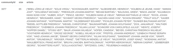
ORDER BY size DESC LIMIT 25Scores of sparse communities, just a few that bubble up to the Top 25. Here’s one that looks to be an all-German club.
Let’s see why. What we’re doing here is taking each of the Artists and charting a shortest path between every other Artist to see possible connections. The APOC procedure apoc.algo.cover only connects Nodes from a list input if they are seen to have a ‘direct’ connection, so that wouldn’t fly here.
CALL gds.louvain.stream('artists&Paintings',
{nodeLabels: ['Artist'],
relationshipTypes: ['ARTIST_SIMILARITY'],
relationshipWeightProperty: 'score',
maxLevels:10, maxIterations:10, includeIntermediateCommunities:false})
YIELD nodeId, communityId, intermediateCommunityIds
WHERE communityId = 3977
WITH COLLECT(gds.util.asNode(nodeId)) AS list
WITH list, range(0, size(list)-1) AS r1, range(0, size(list)-1) AS r2
UNWIND r1 AS i1
UNWIND r2 AS i2
WITH list[i1] AS a, list[i2] AS b
MATCH (a), (b), path = shortestpath((a)-[*]-(b))
WHERE a <> b
RETURN path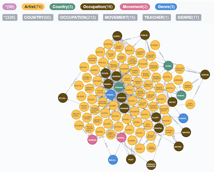
Right, so that brings up a community of German & Dutch Artists belonging to the German Renaissance / Baroque movements sharing varied occupations, which explains why.
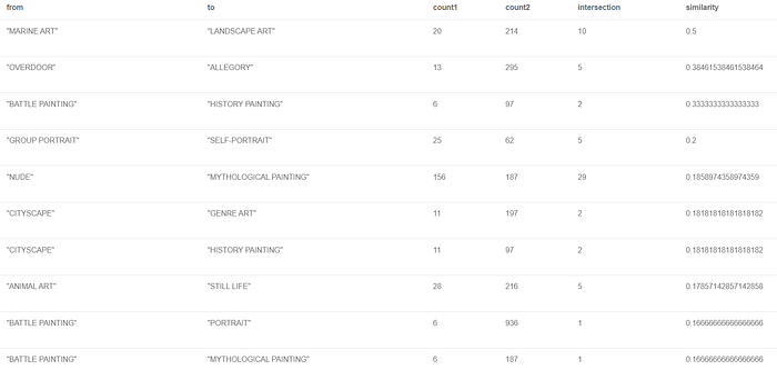
Next, let’s put Overlap Similarity to use with regards to studying Painting Genres and whether they bear allegiance to a possible taxonomy. Here’s a really good post by Dr. Jesús Barrasa@Neo4j on the same.
MATCH (p:Painting)-[:GENRE]->(g)
WITH {item:ID(g), categories: collect(ID(p))} AS paintingData
WITH collect(paintingData) AS paintingData
CALL gds.alpha.similarity.overlap.stream({
  data: paintingData,
  degreeCutoff: 5,
  similarityCutoff: 0.1,
  topK: 3
})
YIELD item1, item2, count1, count2, intersection, similarity
RETURN gds.util.asNode(item1).genre AS from, gds.util.asNode(item2).genre AS to,
       count1, count2, intersection, similarity
ORDER BY similarity DESC LIMIT 50
Not quite impressive but tells you what you can build on with a dataset that’s been well tagged.
Moving on, let’s examine similar Paintings! We’ll reuse the same in-memory projection of Artists with Paintings.
Let’s check a Node Similarity stream for a Painting that features on the Louvre ‘Art of Portraiture’ Album.

CALL gds.nodeSimilarity.stream('artists&Paintings',
{degreeCutoff: 10,
similarityCutoff: 0.25,
topK:10})
YIELD node1, node2, similarity
WHERE node1 <> node2 AND gds.util.asNode(node1).arkID = 'cl010063406'
WITH gds.util.asNode(node1).arkID AS painting1ArkID,
gds.util.asNode(node1).title as painting1Title,
gds.util.asNode(node2).arkID AS painting2ArkID,
gds.util.asNode(node2).title AS painting2Title,
similarity,
[(p:Painting)-[:MOVEMENT]->(m:Movement) WHERE ID(p)=node2|m.movement] AS movement,
[(p:Painting)-[:GENRE]->(g:Genre) WHERE ID(p)=node2|g.genre] AS genre
ORDER BY similarity DESC
RETURN painting1ArkID AS arkID, painting1Title AS title, COLLECT(painting2ArkID) AS similarARKs, COLLECT(painting2Title) AS similarARKTitles,
apoc.coll.toSet(apoc.coll.flatten(COLLECT(movement))) AS movement,
apoc.coll.toSet(apoc.coll.flatten(COLLECT(genre))) AS genre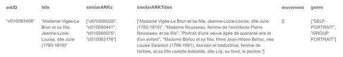

Similar theme, all of them!, in fact the second in the list is the same cast. Amazing, isn’t it? Let’s now look at what a Painting on the very ‘Louvre’ streams, as similar works of art. I picked this one randomly.

CALL gds.nodeSimilarity.stream('artists&Paintings',
{degreeCutoff: 5,
similarityCutoff: 0.2,
topK:10})
YIELD node1, node2, similarity
WHERE node1 <> node2 AND gds.util.asNode(node1).arkID = 'cl010063971'
WITH gds.util.asNode(node1).arkID AS painting1ArkID,
gds.util.asNode(node1).title as painting1Title,
gds.util.asNode(node2).arkID AS painting2ArkID,
gds.util.asNode(node2).title AS painting2Title,
similarity,
[(p:Painting)-[:MOVEMENT]->(m:Movement) WHERE ID(p)=node2|m.movement] AS movement,
[(p:Painting)-[:GENRE]->(g:Genre) WHERE ID(p)=node2|g.genre] AS genre
ORDER BY similarity DESC
RETURN painting1ArkID AS arkID, painting1Title AS title, COLLECT(painting2ArkID) AS similarARKs, COLLECT(painting2Title) AS similarARKTitles,
apoc.coll.toSet(apoc.coll.flatten(COLLECT(movement))) AS movement,
apoc.coll.toSet(apoc.coll.flatten(COLLECT(genre))) AS genre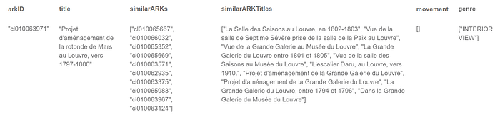
Look at what it identified to be similar! I must say I am mighty pleased with the result. To think there would have been paintings of the Louvre itself!


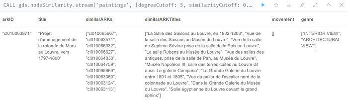
We could create a sub-graph of Paintings alone, leaving out Artists (from not wanting to weigh heavily on lone works from the associated Artist in question), and compare findings.
CALL gds.beta.graph.create.subgraph('paintings', 'artists&Paintings', 'n:Painting OR n:Genre OR n:Movement OR n:Period OR n:Place OR n:Feature OR n:Material OR n:Technique', 'r:GENRE OR r:MOVEMENT OR r:PERIOD OR r:PLACE OR r:FEATURE OR r:MATERIAL OR r:TECHNIQUE')
YIELD graphName, fromGraphName, nodeCount, relationshipCount;
‘Madame Vigée-Le Brun’ brings up additional Paintings that are not quite similar, while the one on ‘Louvre’ just gets better! It has five in common from our last result and five new ones which are simply exquisite.


The next logical step is to stream Louvain and examine clusters of Paintings from our earlier mutated in-memory graph. The results show clusters of religious art, history, nudity, landscape art, still life, emperors / historians, portraiture, mythology, battles fought, murals etc. Now how simple would that make the life of art researchers, restorers, curators, students etc.? For me, that’s a whole treasure unearthed in time. Examples of some clusters;


… and because, I cannot get enough of ‘still life’ (and love rustic kitchens), here’s a few from Chardin’s (muted tones & loose brush strokes) collection that I stumbled upon. There are several Paintings that are tagged as genre ‘still life’ but surprisingly carry anthropomorphized images of animal & marine life. Simply worth a look.

Here’s a cluster of ‘history’ Paintings.


The ‘Coronation of Emperor Napoleon I and coronation of Empress Joséphine in Notre-Dame Cathedral in Paris, December 2, 1804’ on the left above is actually the second largest Painting at the Louvre next to ‘The Wedding Feast at Cana’ that makes for 67.29 sq.mtrs. (724.30 sq.ft.) of canvas. Standing at an unbelievably 33 x 20 ft., the size is no surprise given it were commissioned by the Little General himself and painted by his official painter, Jacques-Louis David. And just so that you know the scale we’re talking of;

Lastly, I pick a cluster of murals.

As always, we’ll be left wanting to do more and honestly, there is far too much to explore in terms of data and Neo4j’s Graph Data Science library. There isn’t enough supporting data at the moment to perform Centrality analysis on say, Artists. I can’t for one seem to put any Path-finding algo to good use for want of weights/geolocations. That said, I’ll continue to look for ways to enrich the current data set and ways to dig in deeper, possibly leveraging other tools within the Neo4j Graph ecosystem. So, stay tuned!